How to use VLOOKUP in Google Sheets
Look up an ID, return the matching entry and fix the range, index and exact-match mistakes behind most VLOOKUP errors.
 Written by PhilisPublished July 20, 2026Last updated July 27, 20269 min
Use =VLOOKUP(E2, A2:C100, 3, FALSE). The lookup ID must be in the first column of the range, index counts columns from the left edge of that range, and FALSE requests an exact match.
VLOOKUP connects two tables through a shared lookup ID. You might use an employee ID to return a department, a product SKU to return a price, or an invoice number to return a payment status.
Most failed lookups are not complicated. The lookup ID is in the wrong column, the index points to the wrong result, or the formula uses approximate matching by accident.
How to use VLOOKUP in Google Sheets
- 01Choose the lookup ID
Use a unique entry, for example an ID, SKU or email, rather than a name that can repeat.
- 02Select the lookup table
Start the range with the column that contains the lookup ID.
- 03Count the result column
The first column in the selected range is 1, the next is 2 and so on.
- 04Use FALSE
Exact matching is the safe default for IDs and labels.
- 05Lock the range
Use absolute references before filling the formula down.
- 06Handle missing IDs
Wrap the lookup with IFNA when a blank or message is more useful than #N/A.
Read the formula from left to right
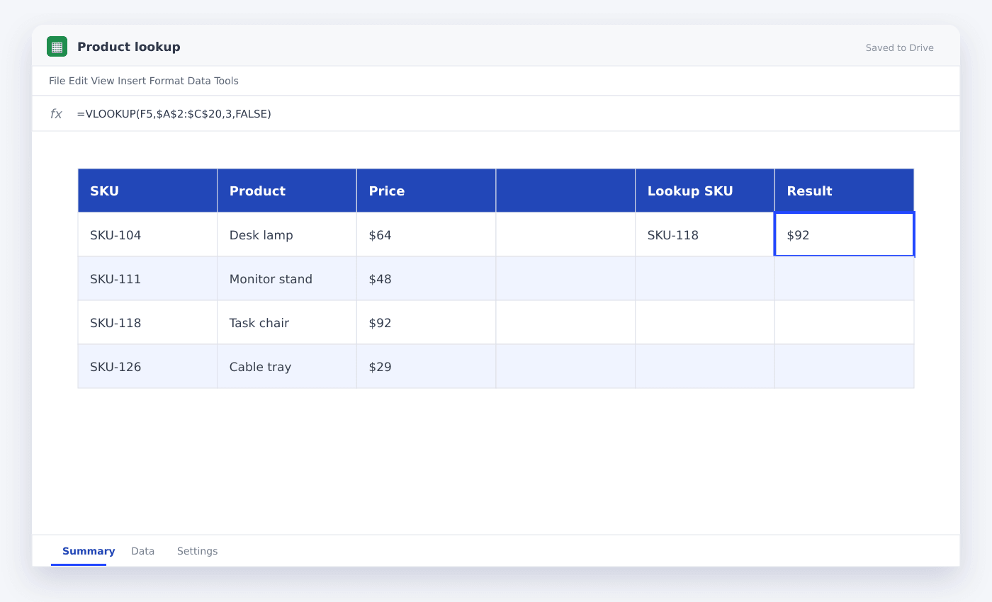
The formula asks Sheets to find E2 in the first column of A2:C100, then return the entry from the third column of the matching row.
The range does not need to start in column A, but the search column must be the leftmost column of the selected range.
=VLOOKUP(E2,$A$2:$C$100,3,FALSE)Fix #N/A and wrong results
#N/A means no exact match was found. Check extra spaces, inconsistent number-versus-text types and whether the lookup ID truly exists.
A believable but wrong result often comes from omitting FALSE. Approximate matching expects sorted data and is rarely appropriate for identifiers.
Know when XLOOKUP is clearer
XLOOKUP uses separate lookup and result ranges, so it can return a column to the left and does not require a numeric index.
Use VLOOKUP when the table is naturally left-to-right and compatibility matters. Use XLOOKUP when the layout may edit or the return column is not to the right.
=XLOOKUP(E2,A2:A100,C2:C100,"Not found")Questions people ask
Why does VLOOKUP return #N/A?+
The lookup ID is missing or stored differently in the two places. Check spaces, punctuation and whether one entry is text while the other is numeric.
Can VLOOKUP look left?+
Not directly. Reorder the selected range or use XLOOKUP or INDEX/MATCH.
Why does the range move when I copy the formula?+
The lookup range is relative. Add dollar signs to lock it, for example $A$2:$C$100.
More from SheetSteps

Google Sheets formula not working? Check these seven things
10 min · Formulas

How to use SUMIF in Google Sheets
8 min · Formulas

How to use IMPORTRANGE in Google Sheets
9 min · AI & automation