INDEX MATCH in Google Sheets: a lookup that works in either direction
Return a field from any column without relying on a left-to-right table layout.
 Written by JosephinePublished June 20, 2026Last updated July 24, 202611 min
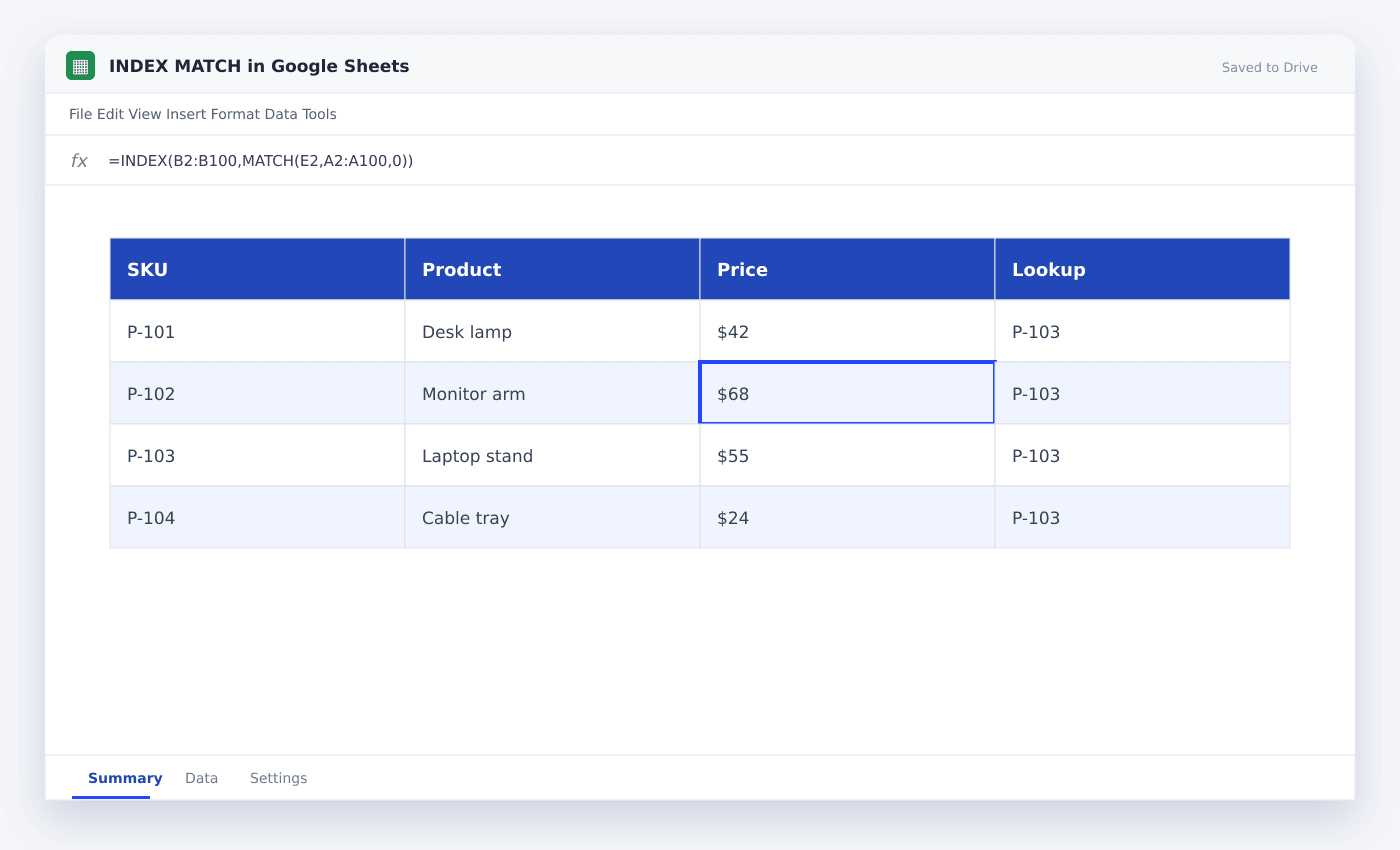
MATCH finds the row number of the lookup item; INDEX returns the entry from that row in another range. Use exact match mode for IDs.
Before you look up a field from any column, set up a clean source range and one result you can check by hand. That gives you a known answer before the sheet grows.
This article shows how to look up a field from any column. The sample sheet uses ordinary rows so you can copy the method into an existing file without rebuilding everything.
INDEX MATCH in Google Sheets: a lookup that works in either direction
- 01Make a safe copy
Duplicate the source tab or file before changing formulas, ranges or formatting.
- 02Set up the source rows
Add the fields needed to look up a field from any column. Keep one record on each row and one field in each column.
- 03Add the method
Enter =INDEX(B2:B100,MATCH(E2,A2:A100,0)) in a test cell and check its first result.
- 04Check a known case
Pick one row whose answer you already know and compare it with the sheet result.
- 05Test the awkward rows
Check blanks, zeros, repeated entries and one row that should not match.
- 06Apply it to the full range
Copy the formula or rule only after the sample cases return the expected result.
Set up the sheet for INDEX MATCH in Google Sheets
Keep the source table rectangular. A single header row, no merged cells and consistent cell types make the work much easier to check.
Place settings, fixed rates or allowed labels on a separate tab. Name them clearly so another person can read the file without tracing every cell.
- Use exact match mode 0
- Keep lookup and return ranges aligned
- Clean spaces in IDs
- Wrap missing matches only when expected
Check the first result before copying it
A result that looks plausible can still be wrong. Work through one row manually, compare it with the Sheet and check every referenced cell.
Next, test a blank row and an unusual row. These two checks catch many range, type and copied-reference mistakes before they spread.
=INDEX(B2:B100,MATCH(E2,A2:A100,0))Keep the file reliable as new rows arrive
Leave input columns visually separate from calculated columns. Protect formulas when several people edit the same file, and keep dropdown lists or settings outside the main table.
Add a short check near the result: row count, unmatched count, last refresh time or a manual spot check. The right check depends on the job, but it should make a bad update easy to notice.
Questions people ask
Why use INDEX MATCH instead of VLOOKUP?+
It can return from a column on either side and does not rely on a fixed column number.
What does the 0 in MATCH mean?+
It requests an exact match.
Can INDEX MATCH return several columns?+
A single formula returns one result, though array methods can return wider ranges.
More from SheetSteps

Google Sheets formula not working? Check these seven things
10 min · Formulas

How to use VLOOKUP in Google Sheets
9 min · Formulas

How to use SUMIF in Google Sheets
8 min · Formulas